Tutorial 3 - plot examples

Demo data for the tutorial can be downloaded from Zenodo

import numpy as np
from matplotlib import pyplot as plt

import SplIsoFind

Construct isoform matrix with relative expression

The create isoform matrix saves a sparse matrix, and corresponding index and column labels to the output folder.

NOTE: this is the same step as we do before calculating Moran’s I.

fn_allinfo = 'data/allinfo_ds.filtered.labeled.gz'
fn_CIDmap = 'data/sample1_barcodeToPos.CellID_ds.tsv.gz'
fn_adata = 'data/sample1_cellbin_adjusted.h5ad'
output = 'data/isoform_matrix'

SplIsoFind.pp.create_isoform_matrix(fn_allinfo,
                      fn_CIDmap,
                      fn_adata,
                      output)

Potentially interesting isoforms (total): 145
Potentially interesting isoforms (novel): 44

We read this sparse matrix to a dense dataframe so we can plot some examples

x, labels = SplIsoFind.pp.sparse2df(input_dir = output)

Plot some examples

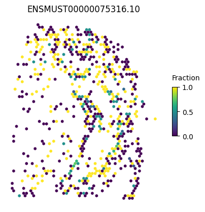
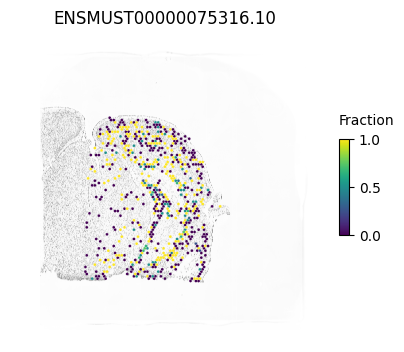
We can make a general plot

isoform = 'ENSMUST00000075316.10'

SplIsoFind.pl.spatial_hexplot(x=x, 
                labels=labels, 
                imarray=None,
                varName=isoform, 
                celltype='', 
                hexsize=350)
plt.show()

We can also plot the staining in the background

from PIL import Image
Image.MAX_IMAGE_PIXELS = 553190400

im_reg = Image.open('data/Sample1_ssDNA_regist.tif')
imarray = np.array(im_reg)

isoform = 'ENSMUST00000075316.10'

SplIsoFind.pl.spatial_hexplot(x=x, 
                labels=labels, 
                imarray=imarray,
                varName=isoform, 
                celltype='', 
                hexsize=350)
plt.show()

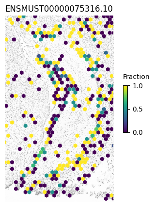
Or we can zoom in a specific region (e.g. the hippocampus)

xlim1=8300
xlim2=14100
ylim1=4450
ylim2=14400

SplIsoFind.pl.spatial_hexplot(x=x, 
                labels=labels, 
                imarray=imarray,
                varName=isoform, 
                celltype='', 
                hexsize=350,
                plot_lim=[xlim1, xlim2, ylim1, ylim2])
plt.show()

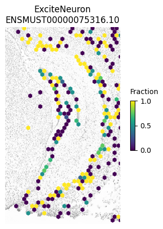
And focus on a specific cell type

SplIsoFind.pl.spatial_hexplot(x=x, 
                labels=labels, 
                imarray=imarray,
                varName=isoform, 
                celltype='ExciteNeuron', 
                hexsize=350,
                plot_lim=[xlim1, xlim2, ylim1, ylim2])
plt.show()

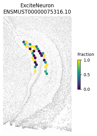
And we can even plot specific regions separately as in Figure 3h.

NOTE: these plots look slightly different from the paper since we downsampled the 4K dataset and not the AE dataset

SplIsoFind.pl.spatial_hexplot(x[(labels['subregion'] == 'DG_ML')], 
                labels[labels['subregion']=='DG_ML'], 
                imarray,
                isoform, 
                celltype='ExciteNeuron', 
                hexsize=350, 
                plot_lim=[xlim1, xlim2, ylim1, ylim2])
plt.show()

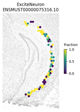
SplIsoFind.pl.spatial_hexplot(x[(labels['subregion'] == 'CA1_ML')], 
                labels[labels['subregion']=='CA1_ML'], 
                imarray,
                isoform, 
                celltype='ExciteNeuron', 
                hexsize=350, 
                plot_lim=[xlim1, xlim2, ylim1, ylim2])
plt.show()

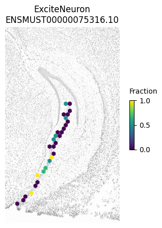
SplIsoFind.pl.spatial_hexplot(x[(labels['subregion'] == 'CA3_ML')], 
                labels[labels['subregion']=='CA3_ML'], 
                imarray,
                isoform, 
                celltype='ExciteNeuron', 
                hexsize=350, 
                plot_lim=[xlim1, xlim2, ylim1, ylim2])
plt.show()