Tutorial 3 - plot examples

Demo data for the tutorial can be downloaded from Zenodo.

import numpy as np
from matplotlib import pyplot as plt

import SplIsoFind

/athena/tilgnerlab/scratch/lim4020/2024_12_20_stereoseq_mousebrain/Reproducibility/SplIsoFind_GitHub/2022_08_15_PSIprediction/envs/SplIsoFind_test/lib/python3.9/site-packages/tqdm_joblib/__init__.py:4: TqdmExperimentalWarning: Using `tqdm.autonotebook.tqdm` in notebook mode. Use `tqdm.tqdm` instead to force console mode (e.g. in jupyter console)
  from tqdm.autonotebook import tqdm

Construct isoform matrix with relative expression

The create isoform matrix saves a sparse matrix, and corresponding index and column labels to the output folder.

NOTE: this is the same step as we do before calculating Moran’s I.

fn_allinfo = 'data/allinfo_ds.filtered.labeled.gz'
fn_CIDmap = 'data/sample1_barcodeToPos.CellID_ds.tsv.gz'
fn_adata = 'data/sample1_cellbin_adjusted.h5ad'
output = 'data/isoform_matrix'

SplIsoFind.pp.create_isoform_matrix(fn_allinfo,
                      fn_CIDmap,
                      fn_adata,
                      output)

Potentially interesting isoforms (total): 145
Potentially interesting isoforms (novel): 44

We read this sparse matrix to a dense dataframe so we can plot some examples

x_sparse, labels, isoforms = SplIsoFind.pp.load_sparse(input_dir = output)

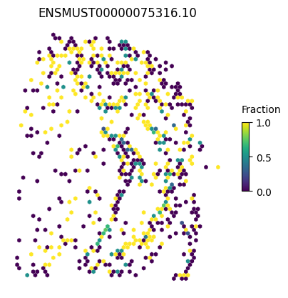
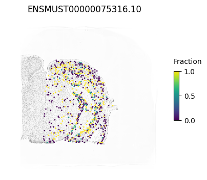
Plot some examples

We can make a general plot

isoform = 'ENSMUST00000075316.10'

SplIsoFind.pl.spatial_hexplot_sparse(x_sparse, 
                                     labels, 
                                     isoforms,
                                     varName=isoform,
                                     imarray=None,
                                     celltype='', 
                                     hexsize=350)
plt.show()

We can also plot the staining in the background

from PIL import Image
Image.MAX_IMAGE_PIXELS = 553190400

im_reg = Image.open('data/Sample1_ssDNA_regist.tif')
imarray = np.array(im_reg)

isoform = 'ENSMUST00000075316.10'

SplIsoFind.pl.spatial_hexplot_sparse(x_sparse, 
                                     labels, 
                                     isoforms,
                                     varName=isoform,
                                     imarray=imarray,
                                     celltype='', 
                                     hexsize=350)

plt.show()

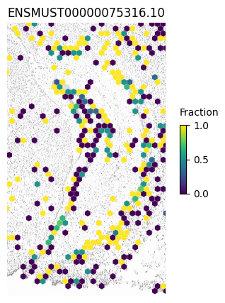
Or we can zoom in a specific region (e.g. the hippocampus)

xlim1=8300
xlim2=14100
ylim1=4450
ylim2=14400

SplIsoFind.pl.spatial_hexplot_sparse(x_sparse, 
                                     labels, 
                                     isoforms,
                                     varName=isoform,
                                     imarray=imarray,
                                     celltype='', 
                                     hexsize=350,
                                     plot_lim=[xlim1, xlim2, ylim1, ylim2])

plt.show()

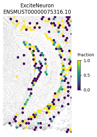
And focus on a specific cell type

SplIsoFind.pl.spatial_hexplot_sparse(x_sparse, 
                                     labels, 
                                     isoforms,
                                     varName=isoform,
                                     imarray=imarray,
                                     hexsize=350,
                                     plot_lim=[xlim1, xlim2, ylim1, ylim2],
                                     celltype='ExciteNeuron')
plt.show()

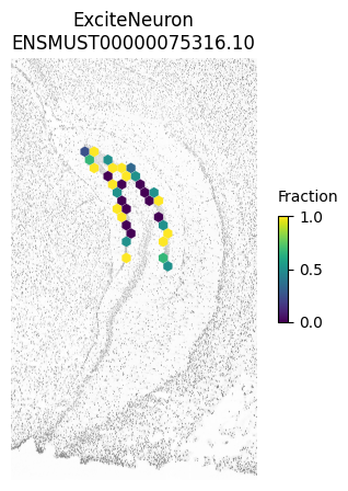
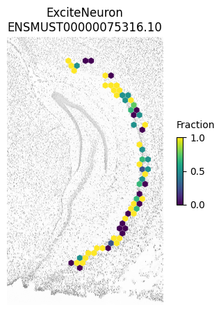
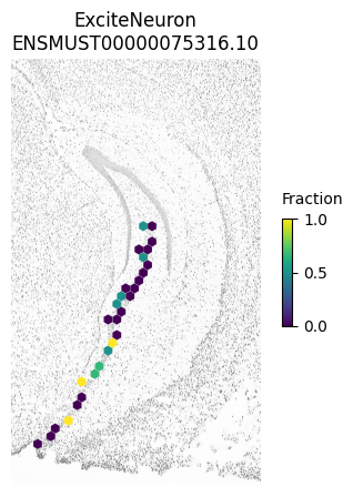
And we can even plot specific regions separately as in Figure 3h.

NOTE: these plots look slightly different from the paper since we downsampled the 4K dataset and not the AE dataset

SplIsoFind.pl.spatial_hexplot_sparse(x_sparse[(labels['subregion'] == 'DG_ML')], 
                                     labels[(labels['subregion'] == 'DG_ML')], 
                                     isoforms,
                                     varName=isoform,
                                     imarray=imarray,
                                     hexsize=350,
                                     plot_lim=[xlim1, xlim2, ylim1, ylim2],
                                     celltype='ExciteNeuron')
plt.show()

SplIsoFind.pl.spatial_hexplot_sparse(x_sparse[(labels['subregion'] == 'CA1_ML')], 
                                     labels[(labels['subregion'] == 'CA1_ML')], 
                                     isoforms,
                                     varName=isoform,
                                     imarray=imarray,
                                     hexsize=350,
                                     plot_lim=[xlim1, xlim2, ylim1, ylim2],
                                     celltype='ExciteNeuron')
plt.show()

SplIsoFind.pl.spatial_hexplot_sparse(x_sparse[(labels['subregion'] == 'CA3_ML')], 
                                     labels[(labels['subregion'] == 'CA3_ML')], 
                                     isoforms,
                                     varName=isoform,
                                     imarray=imarray,
                                     hexsize=350,
                                     plot_lim=[xlim1, xlim2, ylim1, ylim2],
                                     celltype='ExciteNeuron')
plt.show()